L1 and L2 Linear Regression

The goal of this notebook is to validate the optimization code in macaw. For that, we will compare results against sklearn’s linear regression example on the diabetes dataset. See sklearn’s example here: http://scikit-learn.org/stable/auto_examples/linear_model/plot_ols.html#sphx-glr-auto-examples-linear-model-plot-ols-py

%matplotlib inline
import matplotlib.pyplot as plt

from macaw.models import LinearModel
from macaw.objective_functions import L1Norm, L2Norm
from sklearn import datasets
from sklearn.metrics import mean_squared_error, r2_score
import numpy as np

# Load the diabetes dataset
diabetes = datasets.load_diabetes()

# Use only one feature
diabetes_X = diabetes.data[:, np.newaxis, 2]

# Split the data into training/testing sets
diabetes_X_train = diabetes_X[:-20]
diabetes_X_test = diabetes_X[-20:]

# Split the targets into training/testing sets
diabetes_y_train = diabetes.target[:-20]
diabetes_y_test = diabetes.target[-20:]

# Create linear model object
model = LinearModel(diabetes_X_train.reshape(-1))

# Train the model using the training sets
l1norm = L1Norm(y=diabetes_y_train.reshape(-1), model=model)
res_l1 = l1norm.fit(x0=[0., 0.])

# Train the model using the training sets
l2norm = L2Norm(y=diabetes_y_train.reshape(-1), model=model)
res_l2 = l2norm.fit(x0=[0., 0.])

# Make predictions using the testing set
diabetes_y_pred_l1 = LinearModel(diabetes_X_test).evaluate(*res_l1.x)
diabetes_y_pred_l2 = LinearModel(diabetes_X_test).evaluate(*res_l2.x)

print('(L1 Norm) Coefficients: \n', res_l1.x)
print('(L2 Norm) Coefficients: \n', res_l2.x)

(L1 Norm) Coefficients:
 [ 1038.68262063   146.84722666]
(L2 Norm) Coefficients:
 [ 938.23786125  152.91885622]

print("(L1 Norm) Mean squared error: %.2f"
      % mean_squared_error(diabetes_y_test, diabetes_y_pred_l1))
print("(L2 Norm) Mean squared error: %.2f"
      % mean_squared_error(diabetes_y_test, diabetes_y_pred_l2))

(L1 Norm) Mean squared error: 2296.18
(L2 Norm) Mean squared error: 2548.07

print('(L1 Norm) Variance score: %.2f' % r2_score(diabetes_y_test, diabetes_y_pred_l1))
print('(L2 Norm) Variance score: %.2f' % r2_score(diabetes_y_test, diabetes_y_pred_l2))

(L1 Norm) Variance score: 0.52
(L2 Norm) Variance score: 0.47

plt.scatter(diabetes_X_test, diabetes_y_test, color='black')
plt.plot(diabetes_X_test, diabetes_y_pred_l1, color='blue')
plt.plot(diabetes_X_test, diabetes_y_pred_l2, color='red')

[<matplotlib.lines.Line2D at 0x10b05a710>]

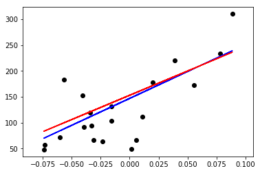
Note that the L1 norm estimator for this particular linear model and dataset presents a smaller mean squared error when compared against the L2 norm estimator. That is because the L1 norm finds the “median model”, and therefore is more robust against outliers, whereas the L2 norm finds the “mean model” which is less robust to the presence of outliers.