Predicting the ages of abalones using Linear Regression
Note: if you don’t now what an abalone is, you might want to educate yourself before proceeding further: https://en.wikipedia.org/wiki/Abalone
In this notebook, we use linear regression to predict the ages of abalones. The dataset used in this short tutorial is available here: https://archive.ics.uci.edu/ml/datasets/abalone.
This dataset provides measurements on physical characteristics of abalones such as length, diameter, height, weight, etc. This physical features will be used to infer the age of abalones.
1. Data Visualization
Let’s load and visualize the dataset using Pandas
In [1]:
import pandas as pd
import numpy as np
np.random.seed(123)
In [2]:
names = ['Sex', 'Length', 'Diameter', 'Height', 'Whole weight',
         'Shucked weight', 'Viscera weight', 'Shell weight', 'Rings']
In [3]:
abalone_df = pd.read_csv('abalone.data', names=names)
In [4]:
abalone_df
Out[4]:
| Sex | Length | Diameter | Height | Whole weight | Shucked weight | Viscera weight | Shell weight | Rings | |
|---|---|---|---|---|---|---|---|---|---|
| 0 | M | 0.455 | 0.365 | 0.095 | 0.5140 | 0.2245 | 0.1010 | 0.1500 | 15 |
| 1 | M | 0.350 | 0.265 | 0.090 | 0.2255 | 0.0995 | 0.0485 | 0.0700 | 7 |
| 2 | F | 0.530 | 0.420 | 0.135 | 0.6770 | 0.2565 | 0.1415 | 0.2100 | 9 |
| 3 | M | 0.440 | 0.365 | 0.125 | 0.5160 | 0.2155 | 0.1140 | 0.1550 | 10 |
| 4 | I | 0.330 | 0.255 | 0.080 | 0.2050 | 0.0895 | 0.0395 | 0.0550 | 7 |
| 5 | I | 0.425 | 0.300 | 0.095 | 0.3515 | 0.1410 | 0.0775 | 0.1200 | 8 |
| 6 | F | 0.530 | 0.415 | 0.150 | 0.7775 | 0.2370 | 0.1415 | 0.3300 | 20 |
| 7 | F | 0.545 | 0.425 | 0.125 | 0.7680 | 0.2940 | 0.1495 | 0.2600 | 16 |
| 8 | M | 0.475 | 0.370 | 0.125 | 0.5095 | 0.2165 | 0.1125 | 0.1650 | 9 |
| 9 | F | 0.550 | 0.440 | 0.150 | 0.8945 | 0.3145 | 0.1510 | 0.3200 | 19 |
| 10 | F | 0.525 | 0.380 | 0.140 | 0.6065 | 0.1940 | 0.1475 | 0.2100 | 14 |
| 11 | M | 0.430 | 0.350 | 0.110 | 0.4060 | 0.1675 | 0.0810 | 0.1350 | 10 |
| 12 | M | 0.490 | 0.380 | 0.135 | 0.5415 | 0.2175 | 0.0950 | 0.1900 | 11 |
| 13 | F | 0.535 | 0.405 | 0.145 | 0.6845 | 0.2725 | 0.1710 | 0.2050 | 10 |
| 14 | F | 0.470 | 0.355 | 0.100 | 0.4755 | 0.1675 | 0.0805 | 0.1850 | 10 |
| 15 | M | 0.500 | 0.400 | 0.130 | 0.6645 | 0.2580 | 0.1330 | 0.2400 | 12 |
| 16 | I | 0.355 | 0.280 | 0.085 | 0.2905 | 0.0950 | 0.0395 | 0.1150 | 7 |
| 17 | F | 0.440 | 0.340 | 0.100 | 0.4510 | 0.1880 | 0.0870 | 0.1300 | 10 |
| 18 | M | 0.365 | 0.295 | 0.080 | 0.2555 | 0.0970 | 0.0430 | 0.1000 | 7 |
| 19 | M | 0.450 | 0.320 | 0.100 | 0.3810 | 0.1705 | 0.0750 | 0.1150 | 9 |
| 20 | M | 0.355 | 0.280 | 0.095 | 0.2455 | 0.0955 | 0.0620 | 0.0750 | 11 |
| 21 | I | 0.380 | 0.275 | 0.100 | 0.2255 | 0.0800 | 0.0490 | 0.0850 | 10 |
| 22 | F | 0.565 | 0.440 | 0.155 | 0.9395 | 0.4275 | 0.2140 | 0.2700 | 12 |
| 23 | F | 0.550 | 0.415 | 0.135 | 0.7635 | 0.3180 | 0.2100 | 0.2000 | 9 |
| 24 | F | 0.615 | 0.480 | 0.165 | 1.1615 | 0.5130 | 0.3010 | 0.3050 | 10 |
| 25 | F | 0.560 | 0.440 | 0.140 | 0.9285 | 0.3825 | 0.1880 | 0.3000 | 11 |
| 26 | F | 0.580 | 0.450 | 0.185 | 0.9955 | 0.3945 | 0.2720 | 0.2850 | 11 |
| 27 | M | 0.590 | 0.445 | 0.140 | 0.9310 | 0.3560 | 0.2340 | 0.2800 | 12 |
| 28 | M | 0.605 | 0.475 | 0.180 | 0.9365 | 0.3940 | 0.2190 | 0.2950 | 15 |
| 29 | M | 0.575 | 0.425 | 0.140 | 0.8635 | 0.3930 | 0.2270 | 0.2000 | 11 |
| ... | ... | ... | ... | ... | ... | ... | ... | ... | ... |
| 4147 | M | 0.695 | 0.550 | 0.195 | 1.6645 | 0.7270 | 0.3600 | 0.4450 | 11 |
| 4148 | M | 0.770 | 0.605 | 0.175 | 2.0505 | 0.8005 | 0.5260 | 0.3550 | 11 |
| 4149 | I | 0.280 | 0.215 | 0.070 | 0.1240 | 0.0630 | 0.0215 | 0.0300 | 6 |
| 4150 | I | 0.330 | 0.230 | 0.080 | 0.1400 | 0.0565 | 0.0365 | 0.0460 | 7 |
| 4151 | I | 0.350 | 0.250 | 0.075 | 0.1695 | 0.0835 | 0.0355 | 0.0410 | 6 |
| 4152 | I | 0.370 | 0.280 | 0.090 | 0.2180 | 0.0995 | 0.0545 | 0.0615 | 7 |
| 4153 | I | 0.430 | 0.315 | 0.115 | 0.3840 | 0.1885 | 0.0715 | 0.1100 | 8 |
| 4154 | I | 0.435 | 0.330 | 0.095 | 0.3930 | 0.2190 | 0.0750 | 0.0885 | 6 |
| 4155 | I | 0.440 | 0.350 | 0.110 | 0.3805 | 0.1575 | 0.0895 | 0.1150 | 6 |
| 4156 | M | 0.475 | 0.370 | 0.110 | 0.4895 | 0.2185 | 0.1070 | 0.1460 | 8 |
| 4157 | M | 0.475 | 0.360 | 0.140 | 0.5135 | 0.2410 | 0.1045 | 0.1550 | 8 |
| 4158 | I | 0.480 | 0.355 | 0.110 | 0.4495 | 0.2010 | 0.0890 | 0.1400 | 8 |
| 4159 | F | 0.560 | 0.440 | 0.135 | 0.8025 | 0.3500 | 0.1615 | 0.2590 | 9 |
| 4160 | F | 0.585 | 0.475 | 0.165 | 1.0530 | 0.4580 | 0.2170 | 0.3000 | 11 |
| 4161 | F | 0.585 | 0.455 | 0.170 | 0.9945 | 0.4255 | 0.2630 | 0.2845 | 11 |
| 4162 | M | 0.385 | 0.255 | 0.100 | 0.3175 | 0.1370 | 0.0680 | 0.0920 | 8 |
| 4163 | I | 0.390 | 0.310 | 0.085 | 0.3440 | 0.1810 | 0.0695 | 0.0790 | 7 |
| 4164 | I | 0.390 | 0.290 | 0.100 | 0.2845 | 0.1255 | 0.0635 | 0.0810 | 7 |
| 4165 | I | 0.405 | 0.300 | 0.085 | 0.3035 | 0.1500 | 0.0505 | 0.0880 | 7 |
| 4166 | I | 0.475 | 0.365 | 0.115 | 0.4990 | 0.2320 | 0.0885 | 0.1560 | 10 |
| 4167 | M | 0.500 | 0.380 | 0.125 | 0.5770 | 0.2690 | 0.1265 | 0.1535 | 9 |
| 4168 | F | 0.515 | 0.400 | 0.125 | 0.6150 | 0.2865 | 0.1230 | 0.1765 | 8 |
| 4169 | M | 0.520 | 0.385 | 0.165 | 0.7910 | 0.3750 | 0.1800 | 0.1815 | 10 |
| 4170 | M | 0.550 | 0.430 | 0.130 | 0.8395 | 0.3155 | 0.1955 | 0.2405 | 10 |
| 4171 | M | 0.560 | 0.430 | 0.155 | 0.8675 | 0.4000 | 0.1720 | 0.2290 | 8 |
| 4172 | F | 0.565 | 0.450 | 0.165 | 0.8870 | 0.3700 | 0.2390 | 0.2490 | 11 |
| 4173 | M | 0.590 | 0.440 | 0.135 | 0.9660 | 0.4390 | 0.2145 | 0.2605 | 10 |
| 4174 | M | 0.600 | 0.475 | 0.205 | 1.1760 | 0.5255 | 0.2875 | 0.3080 | 9 |
| 4175 | F | 0.625 | 0.485 | 0.150 | 1.0945 | 0.5310 | 0.2610 | 0.2960 | 10 |
| 4176 | M | 0.710 | 0.555 | 0.195 | 1.9485 | 0.9455 | 0.3765 | 0.4950 | 12 |
4177 rows × 9 columns
In [5]:
features = ['Length', 'Diameter', 'Height', 'Whole weight',
         'Shucked weight', 'Viscera weight', 'Shell weight']
In [6]:
corr = []
for f in features:
    c = abalone_df[f].corr(abalone_df['Rings'], method='spearman')
    corr.append(c)
In [7]:
corr
Out[7]:
[0.60438533540463257,
 0.62289500509215345,
 0.65771637098609093,
 0.63083195546639859,
 0.53941998208345787,
 0.61434381231405122,
 0.69247456077935632]
In [8]:
import matplotlib.pyplot as plt
%matplotlib inline
In [9]:
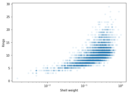
plt.figure(figsize=[7, 5])
plt.semilogx(abalone_df['Shell weight'], abalone_df['Rings'], '*', alpha=.1)
plt.ylabel('Rings')
plt.xlabel('Shell weight')
Out[9]:
<matplotlib.text.Text at 0x118d1c278>
In [10]:
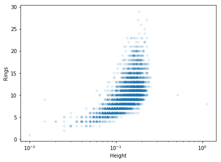
plt.figure(figsize=[7, 5])
plt.semilogx(abalone_df['Height'], abalone_df['Rings'], '*', alpha=.1)
plt.ylabel('Rings')
plt.xlabel('Height')
Out[10]:
<matplotlib.text.Text at 0x119a95d30>
In the column Sex, M, F, and I represent male, female,
and infant, respectively. Nevertheless, we will ignore this feature, and
only consider physical (measurable) features in order to infer ages.
As described in the dataset documentation, the age of an Abalone is
given as Rings + 1.5 (and that’s the label we want to estimate).
Therefore, let’s add an Age label to our dataset:
In [11]:
abalone_df['Age'] = abalone_df['Rings'] + 1.5
2. Model fitting
Let’s use Scikit-learn to split the dataset in training set and testing set:
In [12]:
from sklearn.model_selection import train_test_split
In [13]:
X_train, X_test, y_train, y_test = train_test_split(abalone_df.loc[:, 'Length':'Shell weight'],
                                                    abalone_df['Age'], test_size=.3)
Now, let’s import the objective function L2Norm and the model
LinearModel from macaw:
In [14]:
from macaw.objective_functions import L2Norm
from macaw.models import LinearModel
See https://mirca.github.io/macaw/api/objective_functions.html#macaw.objective_functions for documentation.
Let’s instantiate an object from LinearModel and from L2Norm
passing the labels y_train to the objective function and the
features X_train to the LinearModel:
In [15]:
l2norm = L2Norm(y=np.array(y_train, dtype=float), model=LinearModel(np.array(X_train, dtype=float)))
Let’s use the method fit to get the maximum likelihood weights.
Note that we need to pass an initial estimate for the linear weights and bias of the ``LinearModel``:
In [16]:
res = l2norm.fit(x0=np.zeros(X_train.shape[1] + 1), ftol=0)
The maximum likelihood weights can accessed using the .x attribute:
In [17]:
res.x
Out[17]:
array([ -1.92692825,  13.91714826,  10.18261543,   9.75342147,
       -20.87769625,  -9.89679523,   8.34389868,   4.56176106])
Additionally, we can check the status of the fit and the number of
iterations that it took to converge.
In [18]:
res.status
Out[18]:
'Success: parameters have not changed by 1e-06 since the previous iteration.'
In [19]:
print("Number of iterations needed: {}".format(res.niters))
Number of iterations needed: 127
Now, let’s compute the Mean Squared Error between the model and the labels on the test set:
In [20]:
model_test = LinearModel(X_test)
In [21]:
print('The mean squared error of the model on the test set is {}'
      .format(np.mean((model_test(*res.x) - y_test) ** 2)))
The mean squared error of the model on the test set is 4.867201239148009
3. Comparison against scikit-learn
Let’s compare macaw against scikit-learn:
In [22]:
from sklearn.linear_model import LinearRegression
In [23]:
lreg = LinearRegression()
In [24]:
lreg.fit(X_train, y_train)
/Users/jvmirca/anaconda3/lib/python3.6/site-packages/scipy/linalg/basic.py:1226: RuntimeWarning: internal gelsd driver lwork query error, required iwork dimension not returned. This is likely the result of LAPACK bug 0038, fixed in LAPACK 3.2.2 (released July 21, 2010). Falling back to 'gelss' driver.
  warnings.warn(mesg, RuntimeWarning)
Out[24]:
LinearRegression(copy_X=True, fit_intercept=True, n_jobs=1, normalize=False)
In [25]:
print('The mean squared error of the model on the test set is {}'
      .format(np.mean((lreg.predict(X_test) - y_test) ** 2)))
The mean squared error of the model on the test set is 4.867210207940822
Looks like macaw has a good agreement with sklearn
:)!
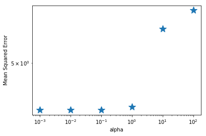
4. Linear Regression with L1 Regularization
In [26]:
from macaw.objective_functions import Lasso
In [31]:
alpha = [1e-3, 1e-2, .1, 1., 10., 100.]
In [32]:
mse = []
for a in alpha:
    lasso = Lasso(y=np.array(y_train, dtype=float), X=np.array(X_train, dtype=float), alpha=a)
    res_lasso = lasso.fit(x0=np.ones(X_train.shape[1] + 1))
    mse.append(np.mean((model_test(*res_lasso.x) - y_test) ** 2))
In [33]:
mse
Out[33]:
[4.867263167748132,
 4.867277337599111,
 4.8679354412745655,
 4.8756478738362805,
 5.09963858836932,
 5.1534303485996595]
In [34]:
plt.loglog(alpha, mse, '*', markersize=15)
plt.ylabel('Mean Squared Error')
plt.xlabel('alpha')
Out[34]:
<matplotlib.text.Text at 0x119aa6048>