Logistic Regression Applied to Classification of Breast Tumors
In this notebook, we use logistic regression to classify breast tumors in two classes, benign or malignant. The dataset used in this short tutorial is available here: https://archive.ics.uci.edu/ml/machine-learning-databases/breast-cancer-wisconsin/. Note: there were a few missing data (label as ‘?’) which were replaced with zeros.
The whole documentation of the dataset can be seen in the
breast-cancer-wisconsin.names file available in the link above.
Nonetheless, I will briefly mention the characteristics of this dataset.
This dataset has nine interger-valued features that biologically
characterizes a given tumor, e.g., size of the cell, clump thickness,
etc. Every sample in the dataset has a label (or class) which
indicates whether the tumor is benign or malignant. Benign samples have
class == 2 whereas malignant samples have class == 4.
1. Data Visualization
Let’s load and visualize the dataset using Pandas
In [1]:
import pandas as pd
import numpy as np
np.random.seed(123)
In [2]:
names = ['Sample code number', 'Clump Thickness', 'Uniformity of Cell Size',
          'Uniformity of Cell Shape', 'Marginal Adhesion', 'Single Epithelial Cell Size',
          'Bare Nuclei', 'Bland Chromatin', 'Normal Nucleoli', 'Mitoses', 'Class']
In [3]:
breast_cancer_df = pd.read_csv('breast-cancer-wisconsin.data', names=names)
In [4]:
breast_cancer_df
Out[4]:
| Sample code number | Clump Thickness | Uniformity of Cell Size | Uniformity of Cell Shape | Marginal Adhesion | Single Epithelial Cell Size | Bare Nuclei | Bland Chromatin | Normal Nucleoli | Mitoses | Class | |
|---|---|---|---|---|---|---|---|---|---|---|---|
| 0 | 1000025 | 5 | 1 | 1 | 1 | 2 | 1 | 3 | 1 | 1 | 2 |
| 1 | 1002945 | 5 | 4 | 4 | 5 | 7 | 10 | 3 | 2 | 1 | 2 |
| 2 | 1015425 | 3 | 1 | 1 | 1 | 2 | 2 | 3 | 1 | 1 | 2 |
| 3 | 1016277 | 6 | 8 | 8 | 1 | 3 | 4 | 3 | 7 | 1 | 2 |
| 4 | 1017023 | 4 | 1 | 1 | 3 | 2 | 1 | 3 | 1 | 1 | 2 |
| 5 | 1017122 | 8 | 10 | 10 | 8 | 7 | 10 | 9 | 7 | 1 | 4 |
| 6 | 1018099 | 1 | 1 | 1 | 1 | 2 | 10 | 3 | 1 | 1 | 2 |
| 7 | 1018561 | 2 | 1 | 2 | 1 | 2 | 1 | 3 | 1 | 1 | 2 |
| 8 | 1033078 | 2 | 1 | 1 | 1 | 2 | 1 | 1 | 1 | 5 | 2 |
| 9 | 1033078 | 4 | 2 | 1 | 1 | 2 | 1 | 2 | 1 | 1 | 2 |
| 10 | 1035283 | 1 | 1 | 1 | 1 | 1 | 1 | 3 | 1 | 1 | 2 |
| 11 | 1036172 | 2 | 1 | 1 | 1 | 2 | 1 | 2 | 1 | 1 | 2 |
| 12 | 1041801 | 5 | 3 | 3 | 3 | 2 | 3 | 4 | 4 | 1 | 4 |
| 13 | 1043999 | 1 | 1 | 1 | 1 | 2 | 3 | 3 | 1 | 1 | 2 |
| 14 | 1044572 | 8 | 7 | 5 | 10 | 7 | 9 | 5 | 5 | 4 | 4 |
| 15 | 1047630 | 7 | 4 | 6 | 4 | 6 | 1 | 4 | 3 | 1 | 4 |
| 16 | 1048672 | 4 | 1 | 1 | 1 | 2 | 1 | 2 | 1 | 1 | 2 |
| 17 | 1049815 | 4 | 1 | 1 | 1 | 2 | 1 | 3 | 1 | 1 | 2 |
| 18 | 1050670 | 10 | 7 | 7 | 6 | 4 | 10 | 4 | 1 | 2 | 4 |
| 19 | 1050718 | 6 | 1 | 1 | 1 | 2 | 1 | 3 | 1 | 1 | 2 |
| 20 | 1054590 | 7 | 3 | 2 | 10 | 5 | 10 | 5 | 4 | 4 | 4 |
| 21 | 1054593 | 10 | 5 | 5 | 3 | 6 | 7 | 7 | 10 | 1 | 4 |
| 22 | 1056784 | 3 | 1 | 1 | 1 | 2 | 1 | 2 | 1 | 1 | 2 |
| 23 | 1057013 | 8 | 4 | 5 | 1 | 2 | 0 | 7 | 3 | 1 | 4 |
| 24 | 1059552 | 1 | 1 | 1 | 1 | 2 | 1 | 3 | 1 | 1 | 2 |
| 25 | 1065726 | 5 | 2 | 3 | 4 | 2 | 7 | 3 | 6 | 1 | 4 |
| 26 | 1066373 | 3 | 2 | 1 | 1 | 1 | 1 | 2 | 1 | 1 | 2 |
| 27 | 1066979 | 5 | 1 | 1 | 1 | 2 | 1 | 2 | 1 | 1 | 2 |
| 28 | 1067444 | 2 | 1 | 1 | 1 | 2 | 1 | 2 | 1 | 1 | 2 |
| 29 | 1070935 | 1 | 1 | 3 | 1 | 2 | 1 | 1 | 1 | 1 | 2 |
| ... | ... | ... | ... | ... | ... | ... | ... | ... | ... | ... | ... |
| 669 | 1350423 | 5 | 10 | 10 | 8 | 5 | 5 | 7 | 10 | 1 | 4 |
| 670 | 1352848 | 3 | 10 | 7 | 8 | 5 | 8 | 7 | 4 | 1 | 4 |
| 671 | 1353092 | 3 | 2 | 1 | 2 | 2 | 1 | 3 | 1 | 1 | 2 |
| 672 | 1354840 | 2 | 1 | 1 | 1 | 2 | 1 | 3 | 1 | 1 | 2 |
| 673 | 1354840 | 5 | 3 | 2 | 1 | 3 | 1 | 1 | 1 | 1 | 2 |
| 674 | 1355260 | 1 | 1 | 1 | 1 | 2 | 1 | 2 | 1 | 1 | 2 |
| 675 | 1365075 | 4 | 1 | 4 | 1 | 2 | 1 | 1 | 1 | 1 | 2 |
| 676 | 1365328 | 1 | 1 | 2 | 1 | 2 | 1 | 2 | 1 | 1 | 2 |
| 677 | 1368267 | 5 | 1 | 1 | 1 | 2 | 1 | 1 | 1 | 1 | 2 |
| 678 | 1368273 | 1 | 1 | 1 | 1 | 2 | 1 | 1 | 1 | 1 | 2 |
| 679 | 1368882 | 2 | 1 | 1 | 1 | 2 | 1 | 1 | 1 | 1 | 2 |
| 680 | 1369821 | 10 | 10 | 10 | 10 | 5 | 10 | 10 | 10 | 7 | 4 |
| 681 | 1371026 | 5 | 10 | 10 | 10 | 4 | 10 | 5 | 6 | 3 | 4 |
| 682 | 1371920 | 5 | 1 | 1 | 1 | 2 | 1 | 3 | 2 | 1 | 2 |
| 683 | 466906 | 1 | 1 | 1 | 1 | 2 | 1 | 1 | 1 | 1 | 2 |
| 684 | 466906 | 1 | 1 | 1 | 1 | 2 | 1 | 1 | 1 | 1 | 2 |
| 685 | 534555 | 1 | 1 | 1 | 1 | 2 | 1 | 1 | 1 | 1 | 2 |
| 686 | 536708 | 1 | 1 | 1 | 1 | 2 | 1 | 1 | 1 | 1 | 2 |
| 687 | 566346 | 3 | 1 | 1 | 1 | 2 | 1 | 2 | 3 | 1 | 2 |
| 688 | 603148 | 4 | 1 | 1 | 1 | 2 | 1 | 1 | 1 | 1 | 2 |
| 689 | 654546 | 1 | 1 | 1 | 1 | 2 | 1 | 1 | 1 | 8 | 2 |
| 690 | 654546 | 1 | 1 | 1 | 3 | 2 | 1 | 1 | 1 | 1 | 2 |
| 691 | 695091 | 5 | 10 | 10 | 5 | 4 | 5 | 4 | 4 | 1 | 4 |
| 692 | 714039 | 3 | 1 | 1 | 1 | 2 | 1 | 1 | 1 | 1 | 2 |
| 693 | 763235 | 3 | 1 | 1 | 1 | 2 | 1 | 2 | 1 | 2 | 2 |
| 694 | 776715 | 3 | 1 | 1 | 1 | 3 | 2 | 1 | 1 | 1 | 2 |
| 695 | 841769 | 2 | 1 | 1 | 1 | 2 | 1 | 1 | 1 | 1 | 2 |
| 696 | 888820 | 5 | 10 | 10 | 3 | 7 | 3 | 8 | 10 | 2 | 4 |
| 697 | 897471 | 4 | 8 | 6 | 4 | 3 | 4 | 10 | 6 | 1 | 4 |
| 698 | 897471 | 4 | 8 | 8 | 5 | 4 | 5 | 10 | 4 | 1 | 4 |
699 rows × 11 columns
In [5]:
features = ['Clump Thickness', 'Uniformity of Cell Size',
            'Uniformity of Cell Shape', 'Marginal Adhesion', 'Single Epithelial Cell Size',
            'Bare Nuclei', 'Bland Chromatin', 'Normal Nucleoli', 'Mitoses']
In [6]:
corr = []
for f in features:
    c = breast_cancer_df[f].corr(breast_cancer_df['Class'], method='spearman')
    corr.append(c)
In [7]:
corr
Out[7]:
[0.68245186937823676,
 0.85548668244535364,
 0.83639412545877556,
 0.7279952033877698,
 0.76273086721512906,
 0.81376763955180775,
 0.74035036553976241,
 0.74382258149235514,
 0.52676617489092259]
Let’s take a look at the distribution of the dataset:
In [8]:
benign_samples = breast_cancer_df[breast_cancer_df['Class'] == 2]
In [9]:
malignant_samples = breast_cancer_df[breast_cancer_df['Class'] == 4]
In [10]:
print("Percentage of benign examples: {}%".format(np.round(len(benign_samples) / len(breast_cancer_df) * 100)))
Percentage of benign examples: 66.0%
In [11]:
print("Percentage of malignant examples: {}%".format(np.round(len(malignant_samples) / len(breast_cancer_df) * 100)))
Percentage of malignant examples: 34.0%
2. Model fitting
Let’s use Scikit-learn to split the dataset in training set and testing set:
In [12]:
from sklearn.model_selection import train_test_split
In [13]:
X_train, X_test, y_train, y_test = train_test_split(breast_cancer_df.loc[:, 'Clump Thickness':'Mitoses'],
                                                    breast_cancer_df['Class'] / 2 - 1, test_size=.3)
Note that I scaled the 'Class' label such that 0 represents
benign sample and 1 represents malignant samples. This has to be
done solely because of the assumptions of the logistic regression
algorithm implemented in macaw.
Now, let’s import the LogisticRegression objective function from
macaw:
In [14]:
from macaw.objective_functions import LogisticRegression
See https://mirca.github.io/macaw/api/objective_functions.html#macaw.objective_functions.LogisticRegression for documentation.
Let’s instantiate an object from LogisticRegression passing the
labels y_train and the features X_train:
In [15]:
logreg = LogisticRegression(y=np.array(y_train, dtype=float), X=np.array(X_train, dtype=float))
Let’s use the method fit to get the maximum likelihood weights.
Note that we need to pass an initial estimate for the linear weights and bias of the ``LogisiticRegression``:
In [16]:
res = logreg.fit(x0=np.zeros(X_train.shape[1] + 1))
The maximum likelihood weights can accessed using the .x attribute:
In [17]:
res.x
Out[17]:
array([  0.6716211 ,  -0.12269987,   0.22323592,   0.37896363,
        -0.06950043,   0.48099004,   0.65926442,   0.25699509,
         0.58662442, -11.18542664])
Additionally, we can check the status of the fit and the number of
iterations that it took to converge.
In [18]:
res.status
Out[18]:
'Success: parameters have not changed by 1e-06 since the previous iteration.'
In [19]:
print("Number of iterations needed: {}".format(res.niters))
Number of iterations needed: 237
Now, let’s compute the accuracy of our model using the test set. For
that we can use the predict method passing the testing samples. This
method outputs the class of each samples:
In [20]:
logreg.predict(np.array(X_test))
Out[20]:
array([ 1.,  0.,  1.,  0.,  0.,  0.,  1.,  0.,  1.,  1.,  0.,  0.,  0.,
        0.,  0.,  1.,  0.,  1.,  0.,  0.,  0.,  0.,  1.,  0.,  1.,  0.,
        0.,  1.,  0.,  1.,  0.,  1.,  0.,  1.,  1.,  0.,  0.,  0.,  0.,
        0.,  0.,  1.,  0.,  1.,  0.,  0.,  0.,  1.,  0.,  1.,  0.,  0.,
        1.,  0.,  0.,  1.,  1.,  0.,  1.,  1.,  1.,  0.,  1.,  0.,  0.,
        0.,  1.,  0.,  0.,  1.,  0.,  0.,  0.,  1.,  0.,  0.,  0.,  0.,
        0.,  1.,  0.,  1.,  1.,  1.,  0.,  0.,  1.,  1.,  0.,  0.,  0.,
        0.,  0.,  0.,  0.,  1.,  1.,  0.,  1.,  0.,  0.,  0.,  1.,  0.,
        1.,  0.,  0.,  1.,  0.,  1.,  0.,  0.,  0.,  0.,  1.,  0.,  0.,
        1.,  1.,  1.,  1.,  0.,  1.,  0.,  1.,  1.,  0.,  0.,  1.,  0.,
        0.,  1.,  1.,  0.,  0.,  0.,  0.,  0.,  0.,  0.,  0.,  1.,  0.,
        0.,  0.,  0.,  0.,  0.,  1.,  0.,  0.,  0.,  1.,  0.,  1.,  1.,
        0.,  0.,  0.,  1.,  1.,  0.,  0.,  1.,  0.,  1.,  0.,  0.,  0.,
        1.,  0.,  1.,  1.,  0.,  1.,  0.,  1.,  0.,  0.,  0.,  0.,  0.,
        0.,  0.,  1.,  1.,  0.,  1.,  0.,  0.,  1.,  1.,  0.,  0.,  1.,
        0.,  0.,  1.,  1.,  0.,  1.,  1.,  0.,  1.,  0.,  0.,  0.,  0.,
        0.,  0.])
Now we can compute the percentage of samples correctly classified:
In [21]:
accuracy = np.round((np.array(y_test) == logreg.predict(np.array(X_test))).sum() / len(np.array(y_test)) * 100, decimals=5)
In [22]:
print('The accuracy of the model is {}%'.format(accuracy))
The accuracy of the model is 96.19048%
3. Comparison against scikit-learn
Let’s compare macaw against scikit-learn:
In [23]:
from sklearn.linear_model import LogisticRegression
In [24]:
logit = LogisticRegression()
In [25]:
logit.fit(X_train, y_train)
Out[25]:
LogisticRegression(C=1.0, class_weight=None, dual=False, fit_intercept=True,
          intercept_scaling=1, max_iter=100, multi_class='ovr', n_jobs=1,
          penalty='l2', random_state=None, solver='liblinear', tol=0.0001,
          verbose=0, warm_start=False)
In [26]:
logit.score(X_test, y_test)
Out[26]:
0.96190476190476193
Looks like macaw has a good agreement with sklearn
:)!
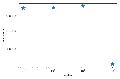
4. Logistic Regression with L1 Regularization
In [27]:
from macaw.objective_functions import L1LogisticRegression
In [28]:
alpha = [.1, 1., 10., 100.]
In [29]:
acc = []
for a in alpha:
    l1logreg = L1LogisticRegression(y=np.array(y_train, dtype=float), X=np.array(X_train, dtype=float), alpha=a)
    res_l1 = l1logreg.fit(x0=np.zeros(X_train.shape[1] + 1) + 1e-1)
    accuracy = np.round((np.array(y_test) == l1logreg.predict(np.array(X_test))).sum() / len(np.array(y_test)) * 100,
                        decimals=5)
    acc.append(accuracy)
In [30]:
acc
Out[30]:
[95.238100000000003,
 95.714290000000005,
 96.666669999999996,
 62.380949999999999]
In [31]:
import matplotlib.pyplot as plt
%matplotlib inline
In [32]:
plt.loglog(alpha, acc, '*', markersize=15)
plt.ylabel('accuracy')
plt.xlabel('alpha')
Out[32]:
<matplotlib.text.Text at 0x112580278>