Robust fitting of linear models using Least Absolute Deviations¶

https://en.wikipedia.org/wiki/Least_absolute_deviations

In [18]:

%matplotlib inline
%config IPython.matplotlib.backend = "retina"
import matplotlib.pyplot as plt
from matplotlib import rcParams
rcParams["figure.dpi"] = 300
rcParams["savefig.dpi"] = 300
rcParams['figure.figsize'] = [7, 5]
rcParams["text.usetex"] = True

In [19]:

import tensorflow as tf
import numpy as np

In [20]:

np.random.seed(123)

In [21]:

from lad import lad

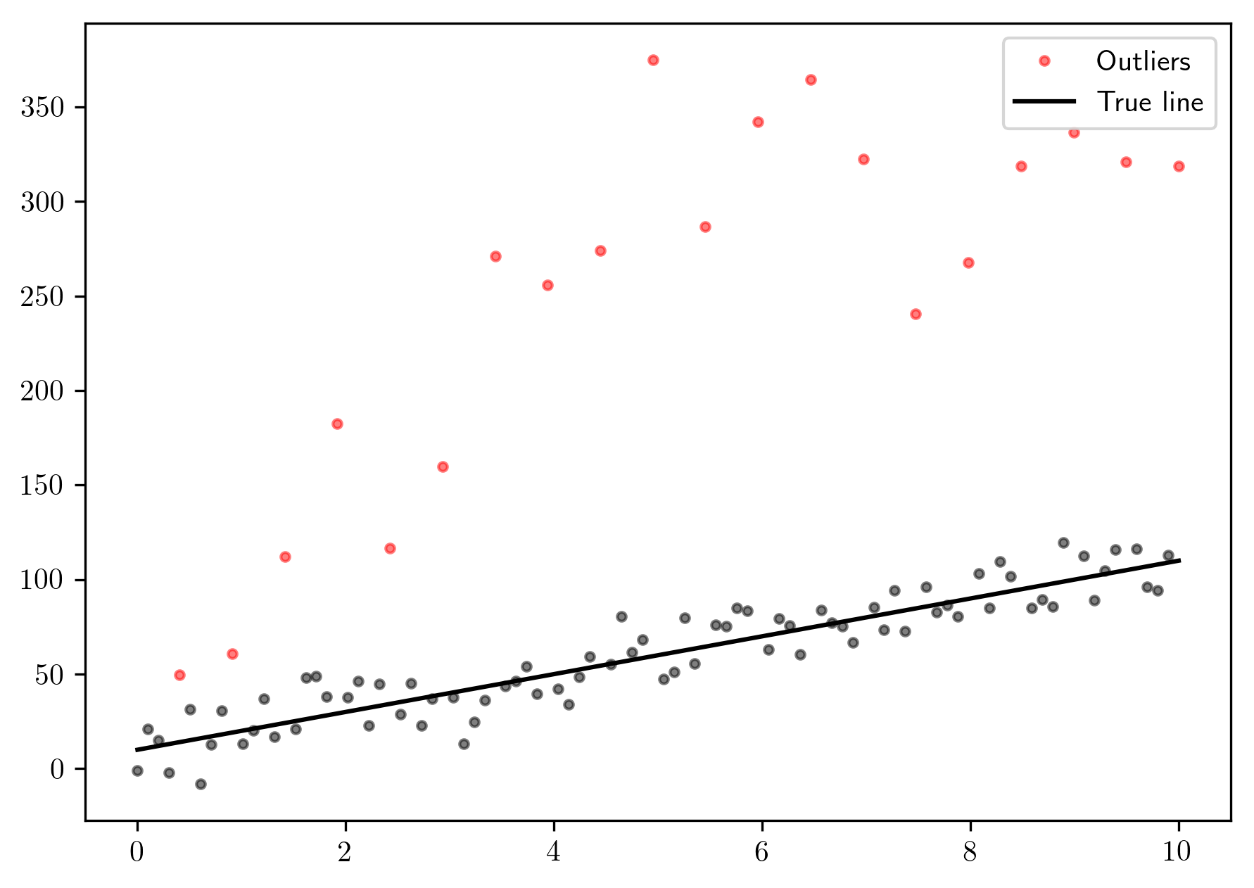
Let’s create some fake data with outliers:

In [22]:

x = np.linspace(0, 10, 100)
noise = 10 * np.random.normal(size=len(x))
y = 10 * x + 10 + noise

In [23]:

mask = np.arange(1, len(x)+1, 1) % 5 == 0
y[mask] = np.linspace(6, 3, len(y[mask])) * y[mask]

In [24]:

plt.plot(x[~mask], y[~mask], 'ok', markersize=3., alpha=.5)
plt.plot(x[mask], y[mask], 'o', markersize=3., color='red', alpha=.5, label='Outliers')
plt.plot(x, 10 * x + 10, 'k', label='True line')
plt.legend()

Out[24]:

<matplotlib.legend.Legend at 0x12c8f2128>

../_images/ipython_notebooks_getting-started_9_1.png

In [25]:

X = np.vstack([x, np.ones(len(x))])

In [26]:

X.shape

Out[26]:

(2, 100)

In [27]:

y.shape

Out[27]:

(100,)

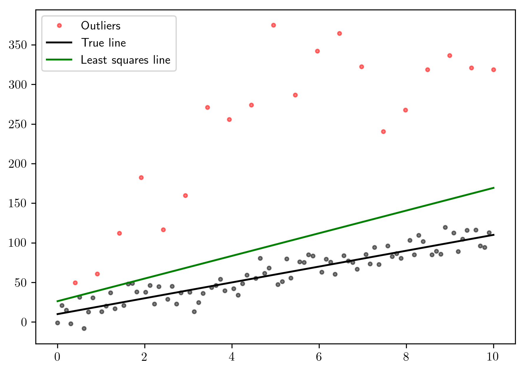
Let’s compute the linear least squares model using tf.matrix_solve_ls:

In [28]:

with tf.Session() as sess:
    X_tensor = tf.convert_to_tensor(X.T, dtype=tf.float64)
    y_tensor = tf.reshape(tf.convert_to_tensor(y, dtype=tf.float64), (-1, 1))
    coeffs = tf.matrix_solve_ls(X_tensor, y_tensor)
    m, b = sess.run(coeffs)

In [29]:

plt.plot(x[~mask], y[~mask], 'ok', markersize=3., alpha=.5)
plt.plot(x[mask], y[mask], 'o', markersize=3., color='red', alpha=.5, label='Outliers')
plt.plot(x, 10 * x + 10, 'k', label="True line")
plt.plot(x, m * x + b, 'g', label="Least squares line")
plt.legend()

Out[29]:

<matplotlib.legend.Legend at 0x12de64e80>

../_images/ipython_notebooks_getting-started_15_1.png

Now let’s use lad to compute the linear model with the least absolute deviations:

In [30]:

l1coeffs, cov = lad(X.T, y, yerr=np.std(y), cov=True)

In [31]:

sess = tf.Session()
m_l1, b_l1 = sess.run(l1coeffs)

And the estimated values are:

In [32]:

m_l1, b_l1

Out[32]:

(array([ 10.5233137]), array([ 13.6857041]))

The uncertanties on the fitted coefficients are:

In [33]:

unc = np.sqrt(np.diag(sess.run(cov)))
unc

Out[33]:

array([ 0.42935153,  3.5996013 ])

In [34]:

plt.plot(x[~mask], y[~mask], 'ok', markersize=3., alpha=.5)
plt.plot(x[mask], y[mask], 'o', markersize=3., color='red', alpha=.5, label='Outliers')
plt.plot(x, 10 * x + 10, 'k', label="True line")
plt.plot(x, m * x + b, 'g', label="Least squares line")
plt.plot(x, m_l1 * x + b_l1, 'blue', label="Least absolute deviations line")
plt.fill_between(x, (m_l1 - 1.96 * unc[0]) * x + b_l1 - 1.96 * unc[1],
                    (m_l1 + 1.96 * unc[0]) * x + b_l1 + 1.96 * unc[1], alpha=.5)
plt.legend()

Out[34]:

<matplotlib.legend.Legend at 0x12f80def0>

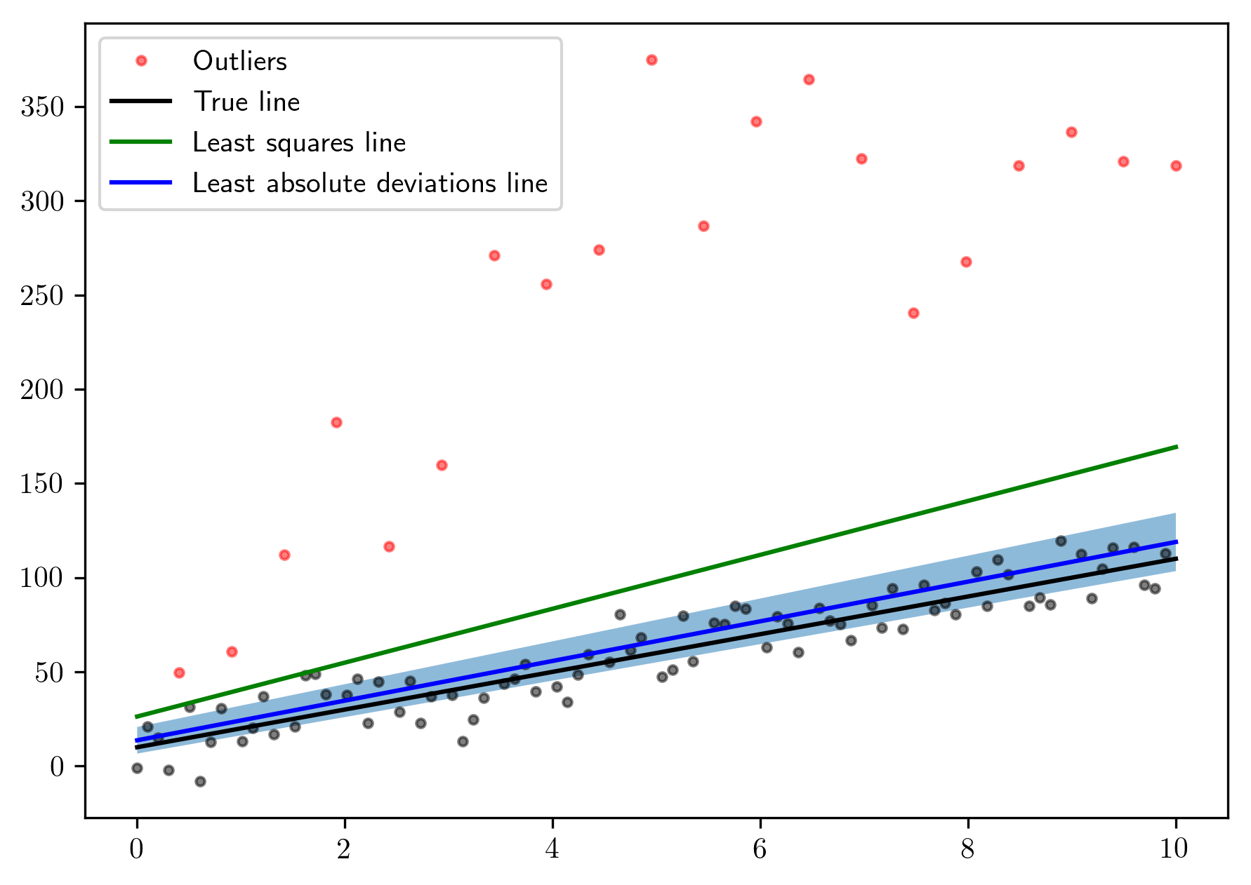
../_images/ipython_notebooks_getting-started_23_1.png

The shaded region is the \(95\%\) confidence interval.